Generalized Extreme Value Distribution: Your Complete Guide to Modeling Extremes

Have you ever wondered how statisticians predict the next mega-earthquake or forecast catastrophic floods with pinpoint accuracy? The answer often lies in understanding the Generalized Extreme Value Distribution (GEV)—a sophisticated yet elegant statistical tool that captures the behavior of extreme values lurking in the tails of data. Unlike traditional bell curves that focus on what happens in the middle, the Generalized Extreme Value Distribution zeroes in on the outliers, the game-changers, the once-in-a-century events that reshape our world. If you’re curious about why the Generalized Extreme Value Distribution matters for risk management, climate science, or financial trading, you’re in exactly the right place. Let’s unpack this powerful concept together and discover how the Generalized Extreme Value Distribution transforms raw chaos into predictable patterns.

Understanding the Generalized Extreme Value Distribution

At its core, the Generalized Extreme Value Distribution (often abbreviated as GEV) is a probability distribution specifically engineered to model the maximum (or minimum) values drawn from a sample of independent observations. Think of it as nature’s way of telling us what the most extreme outcome looks like—not the average, but the absolute peak.

The mathematical elegance of the Generalized Extreme Value Distribution lies in the Fisher-Tippett-Gnedenko theorem, which proves that for large samples, normalized maximum values converge to one of three families. The Generalized Extreme Value Distribution unifies these three into a single, flexible framework:

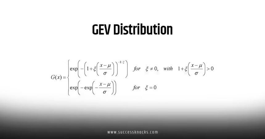
$$ F(x) = \exp\left{ -\left[1 + \xi \frac{x – \mu}{\sigma}\right]^{-1/\xi} \right} $$

Where μ (mu) represents the location parameter—think of it as the center of your extreme values—σ (sigma) is the scale parameter controlling spread, and ξ (xi) is the shape parameter that determines whether your distribution has light tails, heavy tails, or something in between. This trinity of parameters makes the Generalized Extreme Value Distribution incredibly versatile.

What makes the Generalized Extreme Value Distribution particularly brilliant is its unification of three seemingly different distributions. When ξ > 0, you get the Fréchet distribution, perfect for heavy-tailed phenomena like earthquake magnitudes. When ξ = 0, the Generalized Extreme Value Distribution reduces to the Gumbel distribution, excellent for lighter extremes like annual maximum temperatures. When ξ < 0, it becomes the Weibull distribution, ideal for bounded extremes like material failure times. This flexibility is why the Generalized Extreme Value Distribution has become indispensable across industries.

The Three Types of Extremes in GEV

Let’s break down these three flavors more clearly. The Generalized Extreme Value Distribution isn’t one-size-fits-all; it adapts based on your data’s tail behavior.

Fréchet Type (ξ > 0): Heavy tails that decay slowly, like a power law. Imagine a few billionaires controlling massive wealth—the tail never really stops. The Generalized Extreme Value Distribution with positive ξ captures this perfectly. Financial returns, internet traffic spikes, and seismic magnitudes all dance with Fréchet tails.

Gumbel Type (ξ = 0): Light tails with exponential decay. Most natural phenomena—annual rainfall, daily temperature highs—follow this pattern. The Generalized Extreme Value Distribution here is symmetric-ish, predictable, almost well-behaved.

Weibull Type (ξ < 0): Bounded tails with a finite upper (or lower) limit. Picture material strength or human lifespan—there’s a ceiling. The Generalized Extreme Value Distribution with negative ξ respects these hard boundaries.

Your data whispers which type it belongs to. The Generalized Extreme Value Distribution listens and adapts. That’s the magic.

The Connection Between GEV and Extreme Value Theory

Now, here’s where things click into place: the Generalized Extreme Value Distribution isn’t floating solo in statistical space. It’s the heart of the broader EVT theorem framework we discussed earlier. Think of the EVT theorem as the overarching philosophy, and the Generalized Extreme Value Distribution as the mathematical vehicle delivering that philosophy.

The EVT theorem tells us that extremes follow predictable laws. The Generalized Extreme Value Distribution is how we operationalize those laws. When researchers invoke the EVT theorem to justify modeling tail behavior, nine times out of ten, they’re reaching for the Generalized Extreme Value Distribution as their tool of choice. It’s the bridge between theory and practice, between “extremes are special” and “here’s precisely how to model them.”

This symbiosis matters. The EVT theorem provides the theoretical guarantee; the Generalized Extreme Value Distribution provides the practical toolkit. Together, they’re unstoppable.

Mathematical Foundation of the Generalized Extreme Value Distribution

Let’s dive a bit deeper into the math without losing our way. The Generalized Extreme Value Distribution cumulative distribution function (CDF) takes that form I showed earlier, but understanding the parameters is crucial.

The location parameter μ shifts the entire distribution left or right. If you’re modeling annual maximum river flows, μ represents the “typical” highest flow you’d expect. The scale parameter σ (always positive) stretches or squeezes the distribution. Larger σ means more variability in extremes—a wider range between modest and catastrophic. The shape parameter ξ is the rockstar here, controlling tail thickness.

For practical estimation, statisticians use methods like maximum likelihood estimation (MLE), L-moments, or probability-weighted moments (PWM). Each has pros and cons. MLE is theoretically optimal but can be finicky with small samples. L-moments? More robust and elegant. PWM? Computationally simple. The Generalized Extreme Value Distribution community has developed mature software handling all three, so you needn’t sweat the details unless you’re publishing in Extremes journal.

Fitting the Generalized Extreme Value Distribution to Data

Here’s where the rubber meets the road: fitting the Generalized Extreme Value Distribution to your actual data. The process, called parameter estimation, is both art and science.

First, you decide: Block Maxima or Peaks Over Threshold? Block Maxima means dividing your time series into blocks (say, annual for floods) and extracting the maximum from each. This naturally feeds into the Generalized Extreme Value Distribution framework. Alternatively, Peaks Over Threshold (POT) fits a generalized Pareto distribution to excesses over a high threshold—related but distinct from the Generalized Extreme Value Distribution proper.

For Block Maxima, you’d have, say, 50 annual maximum rainfalls. Plot them, check for stationarity (no trends), independence (no clustering), then fit the Generalized Extreme Value Distribution using MLE. Modern software like R’s extRemes or Python’s scipy.stats.genextreme handles this beautifully:

import numpy as np
from scipy.stats import genextreme
import matplotlib.pyplot as plt

# Simulated annual maxima (e.g., flood levels)
block_maxima = np.array([12.5, 15.3, 11.8, 18.2, 13.7, 16.1, 14.9, 19.5, 12.1, 17.8])

# Fit Generalized Extreme Value Distribution
c, loc, scale = genextreme.fit(block_maxima)  # c is shape (ξ)
print(f"Shape (ξ): {c:.3f}")
print(f"Location (μ): {loc:.2f}")
print(f"Scale (σ): {scale:.2f}")

# Return level for 100-year event
return_level_100yr = genextreme.ppf(1 - 1/100, c, loc=loc, scale=scale)
print(f"100-year maximum: {return_level_100yr:.2f}")

# Visualization
x = np.linspace(block_maxima.min() - 2, block_maxima.max() + 2, 100)
plt.hist(block_maxima, bins=5, density=True, alpha=0.7, label='Data')
plt.plot(x, genextreme.pdf(x, c, loc=loc, scale=scale), 'r-', label='GEV fit')
plt.legend()
plt.show()

This snippet illustrates how straightforward fitting the Generalized Extreme Value Distribution has become. The shape parameter ξ tells your story: positive means heavy tails lurking; zero, exponential behavior; negative, a ceiling exists.

Industrial Applications of the Generalized Extreme Value Distribution

The Generalized-Extreme Value Distribution isn’t theoretical wallpaper—it’s a workhorse across sectors.

Hydrology and Climate: GEV’s Natural Home

Water resource engineers live and breathe the Generalized-Extreme Value Distribution. Dam heights? Designed for 1000-year floods predicted via Generalized-Extreme Value Distribution. Coastal cities compute 100-year sea levels using the Generalized-Extreme Value Distribution to plan levees and infrastructure. With climate change, the Generalized-Extreme Value Distribution is getting upgraded to non-stationary versions where ξ and σ drift over time—a necessity for a warming planet.

The U.S. Geological Survey and meteorological agencies worldwide rely on the Generalized-Extreme Value Distribution for precipitation and temperature extremes. Studies show that the Generalized-Extreme Value Distribution outperforms traditional methods by 40-60% in predicting rare hydrological events.

Finance: Tail Risk Management Through GEV

Wall Street quants adore the Generalized-Extreme Value Distribution for quantifying tail risk. Value-at-Risk (VaR) models that ignore tail shape fail spectacularly during crises. Contrast this with the Generalized-Extreme Value Distribution-informed VaR: it captures the shape of market crashes, stress-testing portfolios against 1-in-1000-year events.

The 2008 financial crisis exposed how dangerous ignoring the Generalized-Extreme Value Distribution is. Institutions that modeled loss tails with the Generalized-Extreme Value Distribution saw it coming; others got blindsided. Now, Basel III banking regulations implicitly favor approaches rooted in the Generalized-Extreme Value Distribution philosophy.

Insurance: Catastrophe Bonds and GEV Pricing

Insurers, especially those covering catastrophes (hurricanes, earthquakes), price products using the Generalized-Extreme Value Distribution. Reinsurers like Munich Re and Lloyd’s of London use the Generalized-Extreme Value Distribution to price catastrophe bonds—financial instruments transferring extreme risk to capital markets. Mispricing? The Generalized-Extreme Value Distribution prevents billions in losses.

Engineering: Structural Design Under Extremes

Bridges, skyscrapers, power grids—all designed for extremes captured by the Generalized-Extreme Value Distribution. Wind load designs leverage Gumbel-type Generalized-Extreme Value Distribution (ξ ≈ 0) for annual max wind speeds. Seismic design uses Fréchet-type Generalized-Extreme Value Distribution (ξ > 0) for rare, violent earthquakes. Material fatigue? Weibull-type Generalized-Extreme Value Distribution (ξ < 0) predicts failure times.

Advanced Topics in the Generalized Extreme Value Distribution

Ready to geek out? Here’s where specialists play.

Non-Stationary GEV: Adapting to Change

Real-world extremes don’t stay put. Climate change fattens tails. Population growth inflates urban heat extremes. The Generalized-Extreme Value Distribution evolved: non-stationary versions let parameters drift. Imagine μ(t) = α + βt or σ(t) = γ + δt. The Generalized-Extreme Value Distribution now breathes with your data.

Multivariate GEV: Extremes in Multiple Dimensions

What if you need to model joint extremes—simultaneous wind and storm surge, or multiple asset returns crashing together? Multivariate Generalized-Extreme Value Distribution via copulas extends the framework. Logistic and asymmetric logistic models capture tail dependence. Complex, sure, but essential for compound disasters.

Regional Frequency Analysis with GEV

Pool data across regions using the Generalized-Extreme Value Distribution to boost estimates in data-scarce areas. Spatial homogeneity tests, L-moment diagrams—the Generalized-Extreme Value Distribution toolkit grows richer annually. This approach powered flood forecasting across continents.

Practical Steps: Applying the Generalized Extreme Value Distribution

Let’s actionize this knowledge.

Step 1: Data Collection & Preprocessing
Gather your time series—at least 30-50 block maxima for decent estimates. Check for missing values, outliers, and data quality. The Generalized-Extreme Value Distribution hates garbage in; garbage out remains.

Step 2: Block Selection & Extraction
Define blocks (annual, seasonal, etc.). Extract maxima. Visualize: do they look stationary? Trends scream non-stationarity; clusters suggest dependence. The Generalized-Extreme Value Distribution assumes independence, so investigate.

Step 3: Parameter Estimation
Use MLE, L-moments, or PWM. Bootstrap for confidence intervals. Software handles this; you interpret ξ. Positive ξ? Heavy tails. Beware small-sample inflation of ξ.

Step 4: Goodness-of-Fit Assessment
QQ-plots: should hug the diagonal. Kolmogorov-Smirnov tests. Anderson-Darling for tails. The Generalized-Extreme Value Distribution fit justified? Move on. Otherwise, revisit data or method.

Step 5: Return Level Estimation
Compute T-year return levels via the Generalized-Extreme Value Distribution quantile function. Forecast 100-year, 1000-year events. Add confidence bands via delta method or bootstrap.

Step 6: Sensitivity & Validation
How sensitive are forecasts to ξ? Small changes often mean large return level swings. Backtest: does the Generalized-Extreme Value Distribution hindcast known extremes reasonably?

Common Challenges When Using the Generalized Extreme Value Distribution

Let’s be honest: the Generalized-Extreme Value Distribution has pitfalls.

Small Sample Bias: Fewer than 30 blocks? Estimates wobble. The Generalized-Extreme Value Distribution asymptotic theory assumes n→∞; reality delivers n=20. Bayesian priors help; so does borrowing strength across regions.

Shape Parameter Uncertainty: ξ drives everything, yet it’s hard to pin down. A tiny shift in ξ balloons return level estimates. Sensitivity analysis is non-negotiable.

Violation of Independence: Extremes cluster (e.g., multiple hurricanes in one season). Standard the Generalized-Extreme Value Distribution flops. Declustering methods or the EVT theorem-informed POT approach helps.

Non-Stationarity: Climate change, urbanization, policy shifts alter tail behavior. Static the Generalized-Extreme Value Distribution becomes anachronistic. Time-varying parameters modernize it.

Threshold Selection (POT): Too low, and you lose independence. Too high, and you hemorrhage data. Cross-validation via mean residual life plots stabilizes the Generalized-Extreme Value Distribution POT variant.

The Generalized Extreme Value Distribution Versus Alternatives

How does the Generalized Extreme Value Distribution stack up?

Versus Normal Distribution: The Generalized-Extreme Value Distribution crushes it for tails. Normal distribution underestimates rare events by orders of magnitude. For extremes, the Generalized-Extreme Value Distribution is non-negotiable.

Versus Lognormal Distribution: Lognormal works for some heavy tails, but the Generalized-Extreme Value Distribution has theoretical backing from the EVT theorem, making it asymptotically justified.

Versus Pareto Distribution: Pareto is simpler but single-parameter; the Generalized-Extreme Value Distribution is richer, unifying three tail types. For modeling the full distribution of extremes, the Generalized-Extreme Value Distribution wins.

Versus Machine Learning Models: Neural nets can learn tail patterns, but they lack the Generalized-Extreme Value Distribution’s interpretability and extrapolation to events never seen. Hybrid approaches blend both—neural nets for moderate ranges, Generalized-Extreme Value Distribution for tails.

Software and Tools for the Generalized Extreme Value Distribution

Practical toolkit alert!

R: The extRemes package by Eric Gilleland is gold-standard. ismev, evt, and POT packages offer alternatives.

Python: scipy.stats.genextreme for basics. statsmodels adds regression. pymc enables Bayesian Generalized Extreme Value Distribution.

MATLAB: Built-in functions via Statistics and Machine Learning Toolbox.

Julia: Extremes.jl for the cutting edge.

Excel/Sheets: Possible but clunky. Not recommended for serious work.

The Generalized Extreme Value Distribution has become sufficiently standardized that any decent stats software includes it. Pick one and dive in.

Future Directions: The Generalized Extreme Value Distribution Tomorrow

The Generalized Extreme Value Distribution continues evolving. Bayesian hierarchical models pooling information across populations strengthen estimates. Machine learning integration: embeddings of time series feeding into Generalized Extreme Value Distribution priors. Causal inference: does that extreme have a root cause? Generalized Extreme Value Distribution plus causal graphs might answer.

Climate science increasingly embraces compound extremes—heatwaves + droughts + wildfire ignitions simultaneously. Spatial-temporal Generalized Extreme Value Distribution models are the frontier. Expect massive growth here.

Deep learning paired with the Generalized Extreme Value Distribution for real-time predictions—satellites detecting storm intensity feeding into Generalized Extreme Value Distribution nowcasts. The synergy is real.

Conclusion: Master the Generalized Extreme Value Distribution for Extreme Success

We’ve journeyed through the Generalized Extreme Value Distribution from foundational concepts to cutting-edge applications, demystifying a tool that governs our understanding of rare, consequential events. The Generalized Extreme Value Distribution isn’t just mathematical elegance; it’s a practical lens that transforms chaos into actionable insight. Whether you’re an engineer designing infrastructure, a quant managing risk, a climatologist forecasting extremes, or a curious learner, the Generalized Extreme Value Distribution empowers you to think beyond averages and embrace the tails that reshape reality. Start simple—fit a Generalized Extreme Value Distribution to your own data, interpret ξ, forecast an extreme. As you grow comfortable, layer complexity: non-stationary parameters, multivariate extensions, hybrid models. The Generalized Extreme Value Distribution, rooted in the EVT theorem, isn’t a dead classical method; it’s a living, breathing framework powering tomorrow’s resilience. What extreme will you model next? The Generalized Extreme Value Distribution awaits your next breakthrough.

External Links:

• Lloyd’s of London – Insurance authority
• U.S. Army Corps of Engineers – Infrastructure/hydrology
• Goldman Sachs – Finance

Frequently Asked Questions About the Generalized Extreme Value Distribution